Multiple linear regression in Mathematica

Continuing my slow journey through The Art of Computer Systems Performance Analysis, I've reached chapter 15, "Other Regression Models". I'll cover the first part of the chapter on multiple linear regression models. The definition of multiple linear regression from the textbook:

A multiple linear regression model allows one to predict a response variable $y$ as a function of $k$ predictor variables $x_1,x_2,\ldots,x_k$ using a linear model of the following form:

$$y = b_0 +b_1 x_1 + b_2 x_2 + \cdots + b_k x_k + e$$

Given a sample $(x_{11}, x_{21}, \ldots, x_{k1}, y_1),\ldots,(x_{1n},x_{2n},\ldots,x_{kn},y_n)$ of $n$ observations, the model consists of the following $n$ equations:

$$\begin{aligned} y_1 &= b_0 +b_1 x_{11} + b_2 x_{21} + \cdots + b_k x_{k1} + e_1 \\ y_2 &= b_0 +b_1 x_{12} + b_2 x_{22} + \cdots + b_k x_{k2} + e_2 \\ &\vdots \\ y_n &= b_0 +b_1 x_{1n} + b_n x_{2n} + \cdots + b_k x_{kn} + e_n \\ \end{aligned}$$

In vector notation, we have:

$$\begin{bmatrix} y_1 \\ y_2 \\ \cdot \\ \cdot \\ \cdot \\ y_n \\ \end{bmatrix} = \begin{bmatrix} 1 & x_{11} & x_{21} & \cdots & x_{k1} \\ 1 & x_{12} & x_{22} & \cdots & x_{k2} \\ \cdot & \cdot & \cdot & \cdot & \cdot \\ \cdot & \cdot & \cdot & \cdot & \cdot \\ \cdot & \cdot & \cdot & \cdot & \cdot \\ 1 & x_{1n} & x_{2n} & \cdots & x_{kn} \\ \end{bmatrix} \begin{bmatrix} b_0 \\ b_1 \\ \cdot \\ \cdot \\ \cdot \\ b_k \\ \end{bmatrix} + \begin{bmatrix} e_1 \\ e_2 \\ \cdot \\ \cdot \\ \cdot \\ e_n \\ \end{bmatrix}$$

or

$$\mathbf{y = Xb + e}$$

Box 15.1 contains the formulas relevant to multiple linear regression:

1. Model: $y_i = b_0 +b_1x_{1i} + b_2 x_{2i} + \cdots + b_k x_{ki} + e_i$ or in matrix notation $\mathbf{y = Xb + e}$ where:

   • $b$ is a column vector with $k+1$ elements $b = \{b_0,b_1,\ldots,b_k\}$
   • $y$ is a column vector of $n$ observed values of $y = \{y_1,y_2,\ldots,y_n\}$
   • $X$ is an $n$ row by $k+1$ column matrix whose $(i,j+1)$th element $X_{i,j+1}=1$ if $j=0$ else $x_{ij}$

2. Parameter estimation: $\mathbf{b = (X^TX)^{-1}(X^Ty)}$

3. Allocation of variation:

   • $SSY = \sum_{i=1}^n y^2_i$
   • $SS0 = n \bar y^2$
   • $SST = SST - SS0$
   • $SSE = \{\mathbf{y^Ty - b^TX^Ty}\}$
   • $SSR = SST - SSE$

4. Coefficient of determination: $R^2 = \frac{SSR}{SST} = \frac{SST - SSE}{SST}$

5. Coefficient of multiple correlation $R = \sqrt{\frac{SSR}{SST}}$

6. Degrees of freedom:

   $$\begin{aligned} SST &= SSY &- &SS0 &= &SSR &+ &\;SSE \\ n-1 &= n &- &\; 1 &= &\; k &+ &\;(n - k - 1) \\ \end{aligned}$$

7. Analysis of variance (ANOVA): $MSR=\frac{SSR}{k}$; $MSE=\frac{SSE}{n-k-1}$

   Regression is significant if $MSR/MSE$ is greater than $F_{[1-\alpha;k;n-k-1]}$.

8. Standard deviation of errors: $s_e = \sqrt{MSE}$.

9. Standard error of regression parameters: $s_{b_j} = s_e \sqrt{C_{jj}}$ where $C_{jj}$ is the $j^{th}$ diagonal term of $\mathbf{C = (X^TX)^{-1}}$

10. Prediction: Mean of $m$ future observations:

    $\hat{y}_p = b_0 + b_1 x_1 +b_2 x_{2p} + \cdots + b_k x_{kp}$

    Or in vector notation: $\hat{y}_p = \mathbf{x}^T_p\mathbf{b}$; here $\mathbf{x}^T_p = (1,x_{1p},x_{2p},\ldots,x_{kp})$

11. Standard deviation of predictions: $s_{\hat y_p} = s_e \sqrt{ \frac{1}{m} + \mathbf{x}^T_p(\mathbf{X}^T\mathbf{X})^{-1}\mathbf{x}_p}$

12. All confidence intervals are computed using $t{[1-\alpha/2;n-k-1]}$.

13. Correlation among predictions:

    $$R_{x_1,x_2} = \frac{\sum x_{1i} x_{2i} - n \bar{x_1} \bar{x_2} } {[ \sum x^2_{1i} - n \bar{x}^2_1 ]^{1/2} [\sum x^2_{2i} - n \bar{x}^2_2]^{1/2}}$$

14. Model assumptions

    • Errors are independent and identically distributed normal variations with zero mean.
    • Errors have the same variance for all values of the predictors.
    • Errors are additive.
    • $x_i$'s and $y$ are linearly related.
    • $x_i$'s are nonstochastic (i.e not random) and are measured without error.

15. Visual tests:

    • Scatter plot of errors versus predicted response should not have any trend.
    • The normal quantile-quantile plot of errors should be linear.

Mathematica commands¶

Define our data. Each tuple in the list has form $(x_1, x_2, y)$:

data = {
  {14, 70, 2},
  {16, 75, 5},
  {27, 144, 7},
  {42, 190, 9},
  {39, 210, 10},
  {50, 235, 13},
  {83, 400, 20}
}

Create a linear model:

lm = LinearModelFit[data, {x1, x2}, {x1, x2}]

• ANOVA table:

   lm["ANOVATable"]
  

• Mean of response variable, $\bar y$:

   N[Mean[lm["Response"]]] == 9.42857
  

• SSR, sum of squares due to regression:

   lm["SequentialSumOfSquares"] == {199.845, 0.568796}
  

• Coefficient of determination $R^2$:

   lm["RSquard"] == 0.974236
  

• The predicted response variables for each sample, $\hat y_i$:

   lm["PredictedResponse"] == {3.3, 3.7, 6.8, 9.8, 10.0, 11.9, 20.2}
  

• The residual (error) for each data point in the sample, $e_i$:

   lm["FitResiduals"] == {-1.3, 1.2, 0.15, -0.84, -0.015, 1.02, -0.25}
  

• Regression parameters $\{b_0, b_1, \ldots, b_k\}$:

   lm["BestFitParameters"] == {-0.161, 0.118, 0.0265}
  

• The standard error of the regression parameters:

   lm["ParameterErrors"] == {0.91, 0.19, 0.040}
  

• $b_0 \mp ts_{b_0}$ and $b_1 \mp ts_{b_1}$, the confidence intervals for regression parameters:

  (* Default confidence interval is 0.95. *)
  lm = LinearModelFit[data, {x1, x2}, {x1, x2}, ConfidenceLevel -> 0.95]
  lm["ParameterConfidenceIntervals"]
  (* {{-2.69759, 2.37469}, {-0.416515, 0.652989}, {-0.0858019, 0.138805}} *)
  

• Prediction for observations at 90% confidence level for both many observations and a single observation.

  lm = LinearModelFit[data, {x1, x2}, {x1, x2}, ConfidenceLevel -> 0.9]
  (* for many observations *)
  lm["MeanPredictionBands"] /. {x1 -> 100, x2 -> 550}
  (* {19.5571, 32.919} *)
  
  (* for a single observation *)
  lm["SinglePredictionBands"] /. {x1 -> 100, x2 -> 550}
  (* {19.1207, 33.3554} *)
  

• Mean square values for all regression parameters and the error:

  lm["ANOVATableMeanSquares"] == {199.845, 0.568796, 1.325}
  

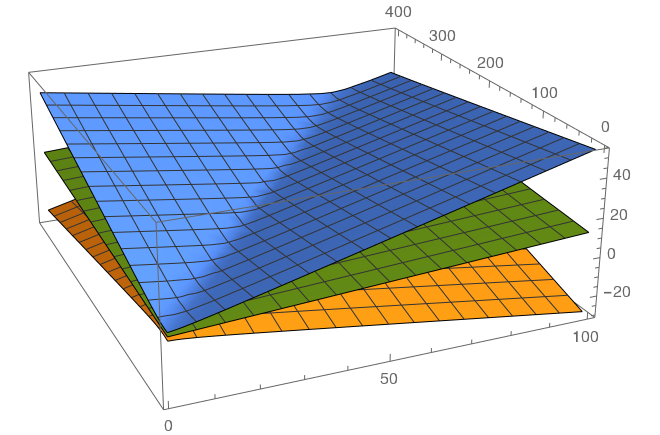
• Plot the mean regression response with the confidence intervals:

  planes = Append[lm["MeanPredictionBands"], lm["BestFit"]];
  Plot3D[planes, {x1, 1, 20}, {x2, 1, 1000}]
  

  

• The correlation matrix, showing $R_{x_ix_j}$ for every pair of $(i,j) < k$

  lm["CorrelationMatrix"] // MatrixForm