Simple linear regression in Mathematica

I'm working my way, slowly, through The Art of Computer Systems Performance Analysis. I've reached the chapter on simple linear regression. Here's how to do simple linear regression in Mathematica.

We'll start by defining our data:

data = {
  {14, 2}, {16, 5}, {27, 7}, {42, 9}, {39, 10}, {50, 13}, {83, 20}
}

We'll create a linear model and show an ANOVA table.

model = LinearModelFit[data, x, x]
model["ANOVATable"]

SS is the sum of squares, the sum of the squared deviations from the expected value.

• SS for x is the sum of squares due to regression (SSR).
• SS for error is the sum of squares due to error (SSE).
• SS for total is the total sum of squares (SST).

MS is mean square, the sum of squares divided by the degrees of freedom.

• MS for x is also SSR because the degrees of freedom for x is 1.
• MS for error is the mean squared error $MSE = SSE / DegreesFreedom$.

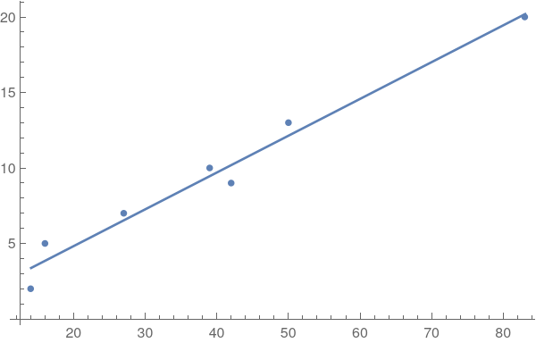
The F-statistic is the mean square of x divided by the mean squared error. Let's plot the data points and regression line:

Show[
  ListPlot[data], 
  Plot[model["BestFit"], {x, Min[First /@ data], Max[First /@ data]}]
]

To get values programmatically:

• $\bar x$, the sample mean of x:

  N[Mean[First /@ data]]
  (* 38.7143 *)
  

• $\bar y$, the sample mean of dependent variables:

  N[Mean[model["Response"]]]
  (* 9.42857 *)
  

• SSY, the sum of squares of the observed, dependent variables:

  Total[#^2 & /@ model["Response"]]
  (* 828 *)
  

• SS0, the sum of squares of the sample mean of the dependent variable:

  N[Length[data]*Mean[model["Response"]]^2]
  (* 622.286 *)
  

• SSR, the sum of squares due to regression:

  model["SequentialSumOfSquares"]
  (* {199.845} *)
  

• $R^2$, the coefficient of determination:

  model["RSquared"]
  (* 0.971471 *)
  

• $b_0$ and $b_1$, the parameters of the regression:

  model["BestFitParameters"]
  (* {-0.00828236, 0.243756} *)
  

• $t_{[1-\alpha/2;n-1]}$, the quantile of a student-t variate at a given significance level $\alpha = 0.1$ and $n - 1 = 6$ degrees of freedom:

  Quantile[StudentTDistribution[6], 0.95]
  (* 1.94318 *)
  

• $\hat y$, the predicted values for each $x$ in the data:

  model["PredictedResponse"]
  (* alternately *)
  model["Function"] /@ First /@ data
  (* {3.40431, 3.89182, 6.57314, 10.2295, 9.49822, 12.1795, 20.2235} *)
  

• $e_i = y_i - \hat y_i$, the error or residuals between the observed and predicted value:

  model["FitResiduals"]
  (* {-1.40, 1.10, 0.42, -1.22, 0.50, 0.82, -0.22} *)
  
  (* squared errors *)
  #^2 & /@ model["FitResiduals"]
  (* {1.97, 1.22, 0.18, 1.51, 0.25, 0.67, 0.049} *)
  

• Table of info about the regression parameters:

  model["ParameterConfidenceIntervalTable"]
  

• $s_{b_0}$ and $s_{b_1}$, the standard errors for the regression parameters:

  model["ParameterErrors"]
  (* {0.831105, 0.0186811} *)
  

• $b_0 \mp ts_{b_0}$ and $b_1 \mp ts_{b_1}$, the confidence intervals for regression parameters:

  (* Default confidence interval is 0.95. *)
  model = LinearModelFit[data, x, x, ConfidenceLevel -> 0.90]
  model["ParameterConfidenceIntervals"]
  (* {{-1.683, 1.66643}, {0.206113, 0.2814}} *)
  

• $\hat y_p$, the mean predicted response for an arbitrary predictor variable $x_p$:

  model["Function"][x_p]
  (* -0.00828236 + 0.243756 x_p *)
  

• $\hat y_p \mp t_{[1-\alpha/2;n-2]}s_{\hat y_p}$, the confidence interval for predicted means using the regression model:

  With many observations such that:

  $$s_{\hat y_p} = s_e \left( \frac{1}{n} + \frac{(x_p- \bar x)^2}{\Sigma x^2 - n \bar x^2} \right)^{1/2}$$

  model = LinearModelFit[data, x, x, ConfidenceLevel -> 0.9]
  model["MeanPredictionBands"] /. x -> 100
  (* {21.9172, 26.8175} *)
  

  Or, with a few observations $m$ such that:

  $$s_{\hat y_p} = s_e \left( \frac{1}{m} + \frac{1}{n} + \frac{(x_p- \bar x)^2}{\Sigma x^2 - n \bar x^2} \right)^{1/2}$$

  Mathematica only has $m=1$, a single prediction, out-of-the-box.

  model = LinearModelFit[data, x, x, ConfidenceLevel -> 0.9]
  model["SinglePredictionBands"] /. x -> 100
  (* {21.0857, 27.649} *)
  

Visual tests for verifying the regression assumptions¶

The mnemonic LINER lists the assumptions necessary for regression. We can check the first four, LINE, using visual tests.

• Linear relationship between $x$ and $y$. Use a scatter plot of the data to verify linearity.

  ListPlot[data]
  

• Independent errors. Prepare a scatter plot of $\epsilon_i$ versus $\hat y_i$. Look for a linear trend.

  ListPlot[
   Transpose[{model["Response"], model["FitResiduals"]}],
   AxesLabel -> {"Predicted response", "Residual"}]
  

• Normally distributed errors. Verify with a histogram of the residuals, looking for a normal distribution. Alternately, verify with a quantile-quantile plot, looking for a linear relationship.

  Histogram[model["FitResiduals"]]
  QuantilePlot[model["FitResiduals"]]
  

• Equal standard deviation (or variance) of errors, known as homoscedasticity. Check with a scatter plot of errors versus the predicted response and check for spread. No spread means the standard deviation is equal.

  ListPlot[
   Transpose[{model["Response"], model["FitResiduals"]}],
   AxesLabel -> {"Predicted response", "Residual"}]