Procella - YouTube’s analytical column store

Procella is a horizontally scalable, eventually consistent, distributed column store leveraging lambda architecture to support both realtime and batch queries [1]. Let’s define those terms one at a time:

• Horizontally scalable means YouTube can spin up more machines and Procella will distribute queries to the new machines automagically.
• Procella doesn't support strong database isolation levels (the I in ACID). Queries support read uncommitted isolation which can cause dirty reads. A dirty read occurs when a transaction sees uncommitted changes from another transaction.
• The lambda architecture means there are two write paths. The first path, called the real-time write path, aims for low latency and writes into an unoptimized row-store that’s immediately available for queries. The second, called the batch write path, ingests large quantities of data into an optimized columnar format. The query path merges changes from both real-time and batch storage to unify results.
• Distributed means the data is sharded across multiple servers.
• A column store refers to how the database physically stores data. See the figure below for how we might store a table with three columns: event_id, time, and path.

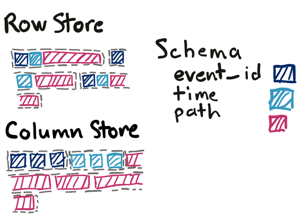
We need a bit more room to explain row stores and column stores. A row store writes data for a single record contiguously. If we’re storing events with three columns event_id, time, and path, a row store writes 1 event_id, then 1 time, then 1 path. Then the row store repeats the process for each row.

A column store writes a single column for many rows contiguously. If we had 5 events, we’d first write five event_ids, then 5 times, then 5 paths. The benefits of a column store are better compression (usually about 10x better) and better locality since all the values for a single column are adjacent. The primary disadvantage is you can’t easily update column stores; you have to rewrite the entire file.

Procella architecture¶

Procella runs on Google infrastructure which has two important consequences. First, storage is completely separate from compute. There are no local disks inside Google. There are only remote procedure calls (RPC). Instead of reading or writing to disk, every read or write is an RPC. Second, binaries run on multi-tenant servers, so a noisy-neighbor can really wreck your day regarding performance. We’ll revisit these points in the optimizations section.

The architecture for Procella is a lambda architecture with two write data flows (realtime and batch), and a single query flow.

The first write path is the batch data flow (in purple). A user creates a file in a supported format (typically through a batch job like an hourly map reduce job). The user sends the file path to the Procella registration server. The registration server checks that the file header matches the SQL schema for the user’s schema. After validation, the file is available for querying. Importantly, Procella doesn't process the file or scan the data other than sanity checking that the schema matches. This approach is a radical departure from most existing row stores. For example, when we write an event into Citus, we create an index on every event definition for that environment.

The second write path is real-time data flow (in blue). Realtime data comes from RPCs or PubSub (similar to Kafka topics). The ingestion server appends the data to a write-ahead log (WAL) and stores the data in memory for querying realtime data. The real-time data flows makes data available for querying in about 1 second. Later, a compaction job will compact the WAL into an optimized columnar format. The compaction job supports user defined transformations including filtering data, aggregating data, and expiring old data. This is a really cool feature. User defined transformations means you can do things like normalize email addresses to all lowercase. The transformations give you a convenient fix for customer-specific customizations.

The query path begins at the root server (in orange). The root server does all the heavy lifting for preparing the query including parsing, query rewrites, planning, plan selection, and plan optimization. The root server then fetches the location of data files from the metadata server. A metadata server is similar to a catalog table which holds the location of all files that make up a table. Oftentimes, the root server can prune files by using zone maps for the file. A zone map is lightweight metadata describing all data in the file. A zone map for a file containing events would include the earliest and latest event time, and the min/max user ID. For example, if a file’s last event time is 2020-01-19, we don’t need to search the file if the query has a predicate like WHERE event_time > '2020-02-01'.

The output of the root server is a physical plan tree. Using trees to distribute large queries to many servers is similar to the approach described in the Dremel (BigQuery) paper [2]. A tree is necessary because the intermediate data for large queries might exceed the resources for a single server. The root server partitions the physical query plan into sub-plans and distributes the sub-plans. Each data server fetches and transforms the data according to the sub-plan.

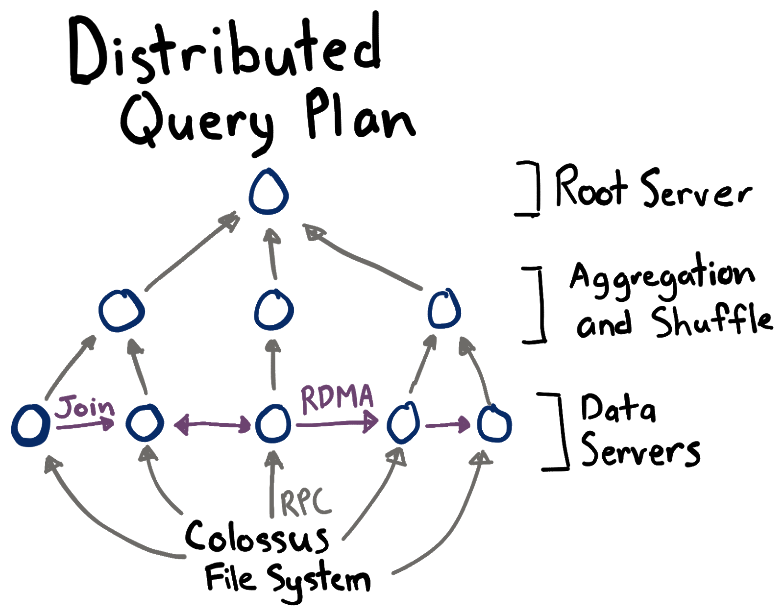
The data servers can communicate among each-other with either RPC or with remote direct memory access (RDMA). After a data server finishes, it sends the results to a parent server for aggregation.

Query evaluation¶

The advantage of a column store for large analytical queries is a combination of four attributes as described by Abadi (think the Knuth of column stores) in The Design and Implementation of Modern Column-Oriented Database Systems [3].

• Vectorized execution: apply functions on an array of values from a single column. In contrast, a row store processes 1 row at time and extracts the column from each row.
• Operation on compressed data: Instead of decompressing data, operate directly on it by using knowledge of the compression scheme. Don’t think GZIP here, think run-length encoding where we can represent the array [3, 3, 3, 3, 8, 8] as [(3, 4), (8, 2)]. With run-length encoding, calculating the count is 4 + 2 = 6.
• Late materialization: the query engine keeps intermediate data in a column format for as long as possible to dramatically speed up aggregations. Materialization means converting columns into rows.
• Database cracking: create indexes just-in-time. The database incrementally sorts columns as a side effect of query processing, e.g. ORDER BY time. With database cracking, we keep the intermediate sorted results for use in following queries. In contrast, row stores require creating indexes ahead of time. Since query patterns change over time, the indexes might not get used. Database cracking ensures indexes are always up to date and match query patterns precisely.

Operation on compressed data¶

Procella leverages adaptive encoding (aka lightweight compression) which is a fancy way of saying it tries a bunch of different encodings and picks the best one. For example, you can use any of the following encodings for an array of integers. Consider the array [3, 4, 4, 4, 0, 0, 9]. Here’s what different encoding would produce.

• Run length encoding: [(3, 1), (4, 3), (0, 2), (9, 1)]
• Delta encoding (the difference from the previous value): [3, 1, 0, 0, -4, 0, 9]
• Frame of reference (the difference from the initial value): [3, 1, 1, 1, -4, -4, 6]

For an array of strings, consider [foo, bar, baz, baz, bar, qux]. Dictionary encoding creates a mapping from a string to an integer:{foo: 0, bar: 1, baz: 2, qux: 3} => [0, 1, 2, 2, 3, 1]. There are all sorts of clever variations on dictionary encoding. Some of my favorites are using prefix compression on the dictionary itself and using a two-level dictionary where each column has its own dictionary and all strings are stored in a global dictionary.

Inverted indexes for experiment IDs¶

Procella relies on database cracking instead of pre-declared indexes. However, Procella supports a single secondary index for arrays of numbers. The use case is to track the results of experiments. Each experiment is represented with an integer ID. A row might have several experiments associated with it, like {row_id: 43, experiments: [543, 778, 901]}. For a query like:

SELECT count(*) FROM events WHERE 543 IN experiments

Procella must check the experiments array of each row. As an optimization, Procella adds an inverted index from an experiment ID to all the rows that contain that experiment. For the example above, the index might look like: {543: [43], 778: [43], 901: [43]}. With this index, we can go to the key 543 and search only those rows. This optimization yielded a 500x speed-up in queries that contained an experiment filter clause.

Optimizations¶

Caching¶

The metadata servers, which contain the mapping of SQL tables to the data files that hold the data, caches the locations of all data files with a 99% hit rate. The paper was unclear, but I’m pretty sure the metadata server uses a three level cache. The source of truth is Spanner, a strongly consistent row store similar to Postgres but magically scalable and expensive. Spanner has a P99 latency of about 500ms. The second level of cache is Bigtable, a key-value store, which has P99 of about 50ms. The final cache is in-memory cache on the server with a latency of about 100ns.

The data servers, which fetch and process data files, cache the data files with a least-recently used scheme to attain a 90% hit rate. Impressively, only 2% of the total data in Procella is stored in memory at any one time. The reason the cache hit rate is high is due to affinity scheduling. Affinity scheduling means the root server will consistently route requests for a file to the same server, improving the hit rate. Notably, the affinity scheduling is loose. If a data server crashes or slows down due to a noisy neighbor, the root server will route the request to a new data server.

Procella optimizes queries with data from running queries instead of maintaining statistics for existing data. Specifically, the root server runs the query on a subset of data to estimate the cardinality and cost of the plan.

Joins¶

Procella supports a number of join algorithms and chooses at query time depending on the number of unique values and sort order. Procella implements joins by transferring information between two data servers or up to a parent server that coordinates the join.

• Broadcast join. If one side of a join has fewer than 100k records, the data server sends all records to other machines doing the join.
• Pre-shuffled. If one side of a join is already partitioned on the join key, have the other side of the join partition itself to match the first side.
• Full-shuffle. If no other join optimization is available, first calculate the number of shards by querying a subset of results. Then each data server sends data to the appropriate server to be joined with the other side.

Tail latency mitigation¶

Okay, remember from up top where I said all reads and writes are really RPCs? This is bad because RPCs are slow, unreliable, and can have exceedingly high tail latency, especially if you send a few thousand at a time. Put simply, if Procella sends out 1000 RPCs, one of those RPCs is likely to be as slow as the 99.9th percentile latency which might be 1-2 orders of magnitude slower than the 50th percentile latency. For more detail on tail latency, I highly recommend The Tail at Scale. Procella uses four techniques to reduce tail latency:

1. Query hedging. To implement query hedging, track the latency of servers in groups of 10 (0-9%, 10-19%, …, 90-100%) ordered by the latency to that server (aka quantiles). If an in-flight query takes longer than the latency of the 70% group, resend the query to a different server. Use whichever query comes back first and discard the slower query.
2. The root server rate limits incoming queries to avoid overwhelming data servers.
3. The root server attaches a priority to each request. Servers maintain separate thread pools for high and low priorities. This ensures intermediate servers serve high priority queries quickly without waiting to process a queue of low priority queries like batch queries.
4. The root server adds intermediate servers to the physical plan tree to help aggregate results if the leaf nodes return many records.